Voltage Sag Analysis#
Introduction#
Voltage sags, also known as voltage dips, are a common power quality issue that can affect electrical equipment performance. They are characterized by a short duration reduction in the RMS voltage, usually lasting from a few milliseconds to a few minutes. In this tutorial, we will explore detection techniques for voltage sags in synchrophasor data using the PredictiveGrid Platform.
Table of Contents#
What are Voltage Sags?#
From the IEEE Standard on Power Quality 1159-2019
A sag is a decrease in rms voltage to between 0.1 pu and 0.9 pu for durations from 0.5 cycles to 1 min.
These are a common type of power quality disturbance that can impact the operation of sensitive equipment.
Key Characteristics#
Duration: 0.5 cycles to ~1 minute
Magnitude: 10% to 90% of nominal voltage 0.9<->0.1 pu
Frequency: Occurrence varies based on system conditions and external factors
Causes of Voltage Sags#
Voltage sags can be caused by various factors, including:
Faults on the power system: Short circuits, lightning strikes, and equipment failures can lead to voltage sags.
Large motor startups: The inrush current required to start large motors can cause a temporary drop in voltage.
Utility grid switching: Switching operations in the utility grid can cause temporary voltage sags.
Measurement and Detection#
To effectively manage voltage sags, it is essential to measure and detect them accurately. Common methods include:
Power quality monitors: Devices that record voltage levels and capture events like sags and swells.
Digital relays: Protection devices that can detect and respond to voltage sags.
RMS Voltage Measurements from PMUs: Can view the RMS voltage timeseries from synchrophasors/other devices and identify for historial or real time detection
Case 1: Distribution PMUs with community solar (Ni4ai dataset)#
The “Sunshine” dataset comes from a distribution system in a sunny climate with significant solar PV generation. The data were collected with micro-PMUs during an early research deployment. There are gaps in the data which correspond to outages as the team was experimenting with different system configurations and wireless communications. When fully connected, each PMU reports data at 120 frames per second on twelve channels: three-phase voltage and current, giving root-mean-square magnitude and phase angle for each.
The six sensor locations correspond to three substation buses, one large PV array, and two university buildings. While all six are within the same city, there are three separate distribution circuits, equipped with two sensors each
1. Connect to the platform and access all voltage streams#
We need to connect to the data timeseries storage platform and then locate the datasets of interest. Note, these systems ran for approximately 18 months at 120Hz so we have a lot of data we can work with!
import matplotlib.pyplot as plt
import pandas as pd
import pingthings as pt
import pyarrow as pa
import pyarrow.compute as pc
import seaborn as sns
from tqdm.notebook import tqdm

sns.set_style("darkgrid")
conn = pt.connect()
print(f"{conn.info() = }")
conn.info() = {'major_version': 5, 'minor_version': 48, 'build': '5.48.0', 'proxy': {'proxy_endpoints': []}}
Filter for voltage mag streams on the A-phase#
Our data exists under the name prefix sunhine/PMU[1-6]
voltage_streams = conn.streams_in_collection(
    "sunshine", is_collection_prefix=True, tags={"unit": "volts"}
)
print(f"{len(voltage_streams) = }")
len(voltage_streams) = 18
Lets get a quick description of some of the main attributes and metadata for these data streams (signals)
For these data streams we just need to check their units, name, collection, and their unique identifier
Each data stream can also have its own set of user-applied metadata called annotations which is a dictionary
streams_summary = [
    {
        "uuid": str(s.uuid),
        "collection": s.collection,
        "name": s.name,
        "unit": s.tags()["unit"],
    }
    for s in voltage_streams
]
streams_summary_df = pd.DataFrame.from_dict(streams_summary, dtype="string").sort_values(
    by=["collection", "name"]
)
streams_summary_df
| uuid | collection | name | unit | |
|---|---|---|---|---|
| 10 | 35bdb8dc-bf18-4523-85ca-8ebe384bd9b5 | sunshine/PMU1 | L1MAG | volts |
| 3 | d4cfa9a6-e11a-4370-9eda-16e80773ce8c | sunshine/PMU1 | L2MAG | volts |
| 11 | b2936212-253e-488a-87f6-a9927042031f | sunshine/PMU1 | L3MAG | volts |
| 5 | e290a69d-1e52-4411-bccd-da7c3f39531c | sunshine/PMU2 | L1MAG | volts |
| 1 | 6ef43c96-9429-48db-9d37-bffd981b4a24 | sunshine/PMU2 | L2MAG | volts |
| 8 | b4920286-9aaa-4ca0-82ac-937e3ff7d8e8 | sunshine/PMU2 | L3MAG | volts |
| 2 | 0295f80f-6776-4384-b563-4582f7256600 | sunshine/PMU3 | L1MAG | volts |
| 13 | 38d62795-6341-4069-96d3-fe74bffcac67 | sunshine/PMU3 | L2MAG | volts |
| 16 | 37539589-88aa-48b7-8cb4-1ea2f32c9e8d | sunshine/PMU3 | L3MAG | volts |
| 12 | 08060a62-04c0-4597-8d2f-7df58e461ba2 | sunshine/PMU4 | L1MAG | volts |
| 9 | 08aac678-a2f5-4a9c-9c18-c569cd414368 | sunshine/PMU4 | L2MAG | volts |
| 15 | 5031918c-346f-4488-9755-b3917153e607 | sunshine/PMU4 | L3MAG | volts |
| 4 | edb36769-f56f-47c5-bbda-a177c424cc4f | sunshine/PMU5 | L1MAG | volts |
| 14 | b4de2e84-7816-4dc7-9702-f1c210586e1c | sunshine/PMU5 | L2MAG | volts |
| 6 | a60aa7aa-9ad1-425b-bb2e-74b42a2cd3e0 | sunshine/PMU5 | L3MAG | volts |
| 0 | d3e9ed52-6db9-4b98-bfda-e1b509148e47 | sunshine/PMU6 | L1MAG | volts |
| 7 | d60fc469-a6da-4c98-8763-fd833293d955 | sunshine/PMU6 | L2MAG | volts |
| 17 | 4833b5e0-ef30-40ed-8db8-352e79d38c28 | sunshine/PMU6 | L3MAG | volts |
We see that for each PMU (e.g. sunshine/PMU1), the voltage streams have a name L{PHASE}MAG where 1 is A, 2 is B…
matches = [  # find the correct stream
    stream
    for stream in voltage_streams
    if stream.collection == "sunshine/PMU1" and stream.name == "L1MAG"
]
assert len(matches) == 1  # make sure there's only one
reference_stream = matches[0]
reference_stream
<pingthings.timeseries.client.Stream at 0x7817c0fc01f0>
# all A-phase streams
a_phase_streams = [s for s in voltage_streams if s.name == "L1MAG" and "PMU3" not in s.collection]
print(f"{len(a_phase_streams) = }")
len(a_phase_streams) = 5
Timeseries data stored in the platform#
In our database, the internal datastructure to store the timeseries is a tree that is indexed on time, the further down the tree you go, the more granular data you encounter. These data are also versioned, so you can pin a computation to a specific version for reproducible queries.
At each level of the tree, we pre-compute and update statistical summary information of the timeseries as data is inserted. If you want to look at all 18 months of the timeseries data and its general trends, you can do so with very little computational and data access penalties.
In addition, this also affords us the following benefits:
We can backfill data at any point, out of order insertions is as fast as regular insertions
a read request for data between
t1andt2is guaranteed to be in sorted order, no additional post processing steps needed for out of order dataReading multiple streams in parallel and combining the results is a very scalable action since each stream is its own tree
We can leverage tree search algorithms and our pre-computed statistical summaries to effictively walk the tree to find our events of interest
def find_sags(
    s: pt.timeseries.Stream,
    normalization_factor: float = 1.0,
    tree_width: int = 52,
    threshold_below_pu: float = 0.9,
    start: int = pt.timeseries.constants.MINIMUM_TIME,
    end: int = pt.timeseries.constants.MAXIMUM_TIME,
    stop_tree_width: int = 30,
    version: int = 0,
) -> list[pa.Table] | None:
    """Recursively walk the tree to find event sags that fit our per-unit threshold."""
    results = []

    # print(f"Searching between {pd.Timestamp(start)} and {pd.Timestamp(end)} at a width of {pt.timeseries.constants.PW[tree_width]}")
    windows = s.windowed_values(
        start=start, end=end, width=pt.timeseries.constants.PW[tree_width], version=version
    )

    min_in_pu = pc.divide(windows["min"], normalization_factor)
    mask_below_thresh = pc.less_equal(min_in_pu, threshold_below_pu)
    mask_min_is_less_than_max = pc.less(windows["min"], windows["max"])
    mask_all = pc.and_(mask_below_thresh, mask_min_is_less_than_max)
    times = pc.filter(windows["time"], mask_all)

    for valid_time in times:
        wstart = valid_time.as_py().value
        wend = wstart + int(2**tree_width)

        # our stop condition
        if tree_width <= stop_tree_width:
            raw_points = s.raw_values(
                wstart - (2**stop_tree_width), wend + (2**stop_tree_width), version
            )
            tmp = pc.divide(raw_points["value"], normalization_factor)
            tmp_tab = pa.table([raw_points["time"], tmp], names=["time", "value"])
            results.append(tmp_tab)
        else:
            sub_results = find_sags(
                s,
                normalization_factor,
                tree_width=tree_width - 1,
                threshold_below_pu=threshold_below_pu,
                start=wstart,
                end=wend,
                stop_tree_width=stop_tree_width,
                version=version,
            )
            if sub_results:
                results.extend(sub_results)

    return results
print(f"{pt.utils.ns_to_datetime(reference_stream.earliest().time) = }")
print(f"{pt.utils.ns_to_datetime(reference_stream.latest().time) = }")
pt.utils.ns_to_datetime(reference_stream.earliest().time) = datetime.datetime(2015, 10, 1, 16, 8, 24, 8333, tzinfo=datetime.timezone.utc)
pt.utils.ns_to_datetime(reference_stream.latest().time) = datetime.datetime(2017, 4, 15, 1, 37, 11, 333333, tzinfo=datetime.timezone.utc)
When choosing a resolution, note that these scale as 2**(point width) ns:
point width |
window size |
|---|---|
52 |
1.71 months |
49 |
6.52 days |
36 |
1.15 minutes |
30 |
1.07 seconds |
A full table of point widths can be found here
Lets walk through the year of 2017, but first lets plot the min, mean, and max of that using a pointwidth of 49
start = pt.utils.to_nanoseconds("2016-01-01")
end = pt.utils.to_nanoseconds("2017-01-01")
tree_width = 49
data = reference_stream.windowed_values(
    start, end, pt.timeseries.constants.PW[tree_width]
).to_pandas()
display(data)
| time | min | mean | max | count | stddev | |
|---|---|---|---|---|---|---|
| 0 | 2015-12-28 06:42:59.920142336+00:00 | 6843.349121 | 7168.283691 | 7262.521484 | 67553994 | 36.483932 |
| 1 | 2016-01-03 19:05:29.873563648+00:00 | 6730.730469 | 7146.284180 | 7236.185547 | 23576416 | 30.368816 |
| 2 | 2016-02-11 21:20:29.594091520+00:00 | 7031.129395 | 7154.589844 | 7244.543945 | 14565545 | 33.561325 |
| 3 | 2016-02-18 09:42:59.547512832+00:00 | 771.582458 | 7151.575684 | 7298.772461 | 67553995 | 32.155090 |
| 4 | 2016-02-24 22:05:29.500934144+00:00 | 6841.355957 | 7156.936035 | 7295.418945 | 67553994 | 36.042336 |
| 5 | 2016-03-02 10:27:59.454355456+00:00 | 6657.979492 | 7154.265137 | 7264.339355 | 67553994 | 36.071171 |
| 6 | 2016-03-08 22:50:29.407776768+00:00 | 6434.283203 | 7156.987305 | 7256.983887 | 67553995 | 37.595371 |
| 7 | 2016-03-15 11:12:59.361198080+00:00 | 4686.440918 | 7150.569336 | 7305.978516 | 67554277 | 37.196758 |
| 8 | 2016-03-21 23:35:29.314619392+00:00 | 6950.402832 | 7154.389648 | 7247.018066 | 67553995 | 37.552750 |
| 9 | 2016-03-28 11:57:59.268040704+00:00 | 6895.064453 | 7162.239258 | 7260.096191 | 67553994 | 35.820419 |
| 10 | 2016-04-04 00:20:29.221462016+00:00 | 7017.028320 | 7161.456055 | 7301.885254 | 67553994 | 35.994030 |
| 11 | 2016-04-10 12:42:59.174883328+00:00 | 6825.371094 | 7152.109863 | 7284.200684 | 66929118 | 34.552238 |
| 12 | 2016-04-17 01:05:29.128304640+00:00 | 7006.658691 | 7154.467773 | 7288.672852 | 67554633 | 38.513111 |
| 13 | 2016-04-23 13:27:59.081725952+00:00 | 6946.461426 | 7162.595703 | 7258.621582 | 67554305 | 30.351898 |
| 14 | 2016-04-30 01:50:29.035147264+00:00 | 6931.153320 | 7164.866699 | 7298.011230 | 67287216 | 36.523064 |
| 15 | 2016-05-06 14:12:58.988568576+00:00 | 6580.954102 | 7164.040527 | 7300.862305 | 67417383 | 39.368473 |
| 16 | 2016-05-13 02:35:28.941989888+00:00 | 6904.077148 | 7153.435547 | 7280.838379 | 67433250 | 34.433182 |
| 17 | 2016-05-19 14:57:58.895411200+00:00 | 6796.833984 | 7160.814941 | 7257.706543 | 67481123 | 32.911831 |
| 18 | 2016-05-26 03:20:28.848832512+00:00 | 6869.313477 | 7161.872559 | 7264.391113 | 67467355 | 34.305164 |
| 19 | 2016-06-01 15:42:58.802253824+00:00 | 7044.268066 | 7150.854980 | 7286.551270 | 12435504 | 38.305382 |
| 20 | 2016-06-14 16:27:58.709096448+00:00 | 6987.609375 | 7187.986816 | 7319.545898 | 4265839 | 33.658150 |
| 21 | 2016-06-21 04:50:28.662517760+00:00 | 7016.422363 | 7156.465820 | 7281.102539 | 67258327 | 42.842468 |
| 22 | 2016-06-27 17:12:58.615939072+00:00 | 7019.675781 | 7158.371582 | 7325.371582 | 67418630 | 39.184334 |
| 23 | 2016-07-04 05:35:28.569360384+00:00 | 6964.914551 | 7161.475586 | 7293.490723 | 67554257 | 37.822296 |
| 24 | 2016-07-10 17:57:58.522781696+00:00 | 6939.099121 | 7167.416504 | 7282.670410 | 67472038 | 37.911224 |
| 25 | 2016-07-17 06:20:28.476203008+00:00 | 6710.916992 | 7165.017578 | 7294.763184 | 67553994 | 40.225117 |
| 26 | 2016-07-23 18:42:58.429624320+00:00 | 6905.503906 | 7174.147949 | 7290.334473 | 67554245 | 38.372890 |
| 27 | 2016-07-30 07:05:28.383045632+00:00 | 5558.574219 | 7163.209473 | 7294.157715 | 67230715 | 39.522358 |
| 28 | 2016-08-05 19:27:58.336466944+00:00 | 6865.908203 | 7163.151855 | 7277.530273 | 67009434 | 37.245747 |
| 29 | 2016-08-12 07:50:28.289888256+00:00 | 5780.056641 | 7167.132324 | 7307.212891 | 67041715 | 40.181225 |
| 30 | 2016-08-18 20:12:58.243309568+00:00 | 6915.653809 | 7161.263184 | 7284.014648 | 67235994 | 44.174938 |
| 31 | 2016-08-25 08:35:28.196730880+00:00 | 6905.443848 | 7153.177246 | 7277.511719 | 67261915 | 42.096008 |
| 32 | 2016-08-31 20:57:58.150152192+00:00 | 6720.514160 | 7165.144531 | 7279.988770 | 67055994 | 39.953091 |
| 33 | 2016-09-07 09:20:28.103573504+00:00 | 6635.283203 | 7163.291992 | 7290.200684 | 67373154 | 39.882545 |
| 34 | 2016-09-13 21:42:58.056994816+00:00 | 6899.274414 | 7161.347168 | 7290.335938 | 67292275 | 40.514523 |
| 35 | 2016-09-20 10:05:28.010416128+00:00 | 6392.520996 | 7157.802246 | 7318.228516 | 67266723 | 39.112907 |
| 36 | 2016-09-26 22:27:57.963837440+00:00 | 7022.315918 | 7165.664062 | 7300.725098 | 67240451 | 41.436214 |
| 37 | 2016-10-03 10:50:27.917258752+00:00 | 6944.974121 | 7160.436523 | 7290.101562 | 67553994 | 40.870972 |
| 38 | 2016-10-09 23:12:57.870680064+00:00 | 5955.321289 | 7151.042969 | 7268.437500 | 67553994 | 41.210709 |
| 39 | 2016-10-16 11:35:27.824101376+00:00 | 6901.324219 | 7157.287109 | 7276.021973 | 53614102 | 33.036419 |
| 40 | 2016-10-22 23:57:57.777522688+00:00 | 5097.312988 | 7148.091797 | 7255.719727 | 66125044 | 35.632080 |
| 41 | 2016-10-29 12:20:27.730944+00:00 | 6889.393066 | 7162.962891 | 7266.520508 | 67553995 | 32.416542 |
| 42 | 2016-11-05 00:42:57.684365312+00:00 | 7027.067383 | 7156.406250 | 7283.453613 | 67554116 | 40.484756 |
| 43 | 2016-11-11 13:05:27.637786624+00:00 | 6561.685059 | 7160.247559 | 7270.737305 | 67553994 | 34.567955 |
| 44 | 2016-11-18 01:27:57.591207936+00:00 | 7022.316895 | 7155.961914 | 7247.269043 | 67553995 | 35.379372 |
| 45 | 2016-11-24 13:50:27.544629248+00:00 | 6753.344238 | 7153.865723 | 7258.376953 | 67553994 | 29.264280 |
| 46 | 2016-12-01 02:12:57.498050560+00:00 | 6591.234863 | 7164.776855 | 7281.747559 | 67553995 | 34.874657 |
| 47 | 2016-12-07 14:35:27.451471872+00:00 | 6891.418457 | 7160.816406 | 7265.049316 | 67553994 | 32.994476 |
| 48 | 2016-12-14 02:57:57.404893184+00:00 | 7022.719238 | 7156.711426 | 7261.208008 | 67553994 | 34.202499 |
| 49 | 2016-12-20 15:20:27.358314496+00:00 | 6501.114258 | 7162.756836 | 7282.777344 | 67553995 | 37.336090 |
Each of these summary points we read are based on approximately 67,553,994 raw measurements!
data[data["min"] / data["mean"].mean() < 0.9]
| time | min | mean | max | count | stddev | |
|---|---|---|---|---|---|---|
| 3 | 2016-02-18 09:42:59.547512832+00:00 | 771.582458 | 7151.575684 | 7298.772461 | 67553995 | 32.155090 |
| 6 | 2016-03-08 22:50:29.407776768+00:00 | 6434.283203 | 7156.987305 | 7256.983887 | 67553995 | 37.595371 |
| 7 | 2016-03-15 11:12:59.361198080+00:00 | 4686.440918 | 7150.569336 | 7305.978516 | 67554277 | 37.196758 |
| 27 | 2016-07-30 07:05:28.383045632+00:00 | 5558.574219 | 7163.209473 | 7294.157715 | 67230715 | 39.522358 |
| 29 | 2016-08-12 07:50:28.289888256+00:00 | 5780.056641 | 7167.132324 | 7307.212891 | 67041715 | 40.181225 |
| 35 | 2016-09-20 10:05:28.010416128+00:00 | 6392.520996 | 7157.802246 | 7318.228516 | 67266723 | 39.112907 |
| 38 | 2016-10-09 23:12:57.870680064+00:00 | 5955.321289 | 7151.042969 | 7268.437500 | 67553994 | 41.210709 |
| 40 | 2016-10-22 23:57:57.777522688+00:00 | 5097.312988 | 7148.091797 | 7255.719727 | 66125044 | 35.632080 |
Lets walk through the year of data! And use a stopping window size of 1.07 seconds
norm_factor = data["mean"].mean()
sags = find_sags(
    s=reference_stream,
    start=start,
    end=end,
    normalization_factor=norm_factor,
    stop_tree_width=30,
    tree_width=52,
    version=0,
    threshold_below_pu=0.90,
)
counter = 0
for result in sags:
    counter += 1
    print(f"Found {counter} sag! between {result['time'][0]} and {result['time'][-1]}")
Found 1 sag! between 2016-02-18 09:54:12.791666+00:00 and 2016-02-18 09:54:15.999999+00:00
Found 2 sag! between 2016-02-18 09:54:13.858333+00:00 and 2016-02-18 09:54:17.074999+00:00
Found 3 sag! between 2016-03-11 23:37:22.816666+00:00 and 2016-03-11 23:37:26.033333+00:00
Found 4 sag! between 2016-03-15 22:16:57.333333+00:00 and 2016-03-15 22:17:00.549999+00:00
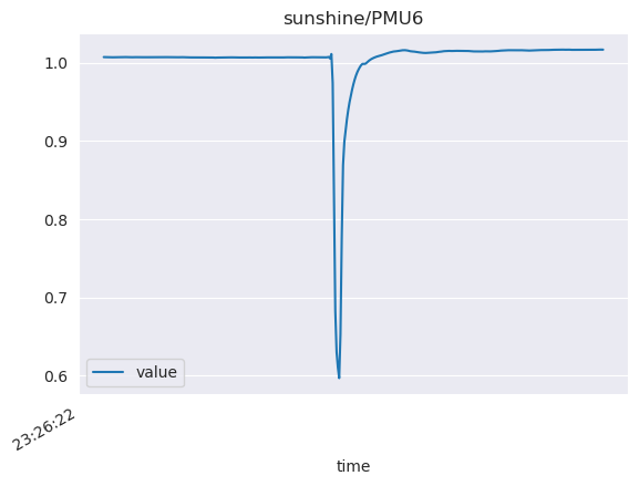
Found 5 sag! between 2016-03-15 23:26:22.374999+00:00 and 2016-03-15 23:26:25.591666+00:00
Found 6 sag! between 2016-08-02 23:05:02.624999+00:00 and 2016-08-02 23:05:05.841666+00:00
Found 7 sag! between 2016-08-02 23:05:03.699999+00:00 and 2016-08-02 23:05:06.916666+00:00
Found 8 sag! between 2016-08-16 18:45:06.758333+00:00 and 2016-08-16 18:45:09.966666+00:00
Found 9 sag! between 2016-09-26 13:11:10.641666+00:00 and 2016-09-26 13:11:13.849999+00:00
Found 10 sag! between 2016-10-14 11:03:59.699999+00:00 and 2016-10-14 11:04:02.908333+00:00
Found 11 sag! between 2016-10-24 04:58:10.583333+00:00 and 2016-10-24 04:58:13.799999+00:00
Found 12 sag! between 2016-10-24 13:31:51.266666+00:00 and 2016-10-24 13:31:54.483333+00:00
Found 13 sag! between 2016-10-24 13:49:17.091666+00:00 and 2016-10-24 13:49:20.308333+00:00
Found 14 sag! between 2016-10-24 14:05:23.458333+00:00 and 2016-10-24 14:05:26.674999+00:00
Found 15 sag! between 2016-10-24 19:13:00.008333+00:00 and 2016-10-24 19:13:03.224999+00:00
Found 16 sag! between 2016-10-24 22:45:59.683333+00:00 and 2016-10-24 22:46:02.899999+00:00
result.to_pandas().set_index("time").plot()
<Axes: xlabel='time'>
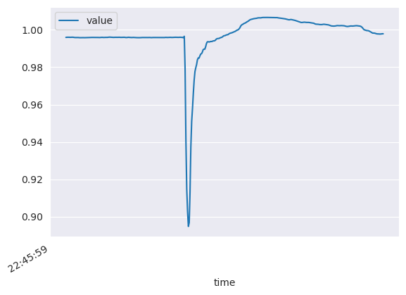
result.to_pandas()["value"].min()
np.float32(0.89475393)
Lets do this for all A phase voltage streams!
result_dict = dict()
start = pt.utils.to_nanoseconds("2016-01-01")
end = pt.utils.to_nanoseconds("2017-01-01")
for stream in tqdm(a_phase_streams, unit="stream"):
    print(stream.collection)
    norm_factor = pc.mean(
        stream.windowed_values(start, end, width=pt.timeseries.constants.PW[52])["mean"]
    ).as_py()
    print(f"{norm_factor = }")
    result_dict[str(stream.collection)] = find_sags(
        stream,
        start=start,
        end=end,
        tree_width=52,
        stop_tree_width=30,
        threshold_below_pu=0.9,
        normalization_factor=norm_factor,
        version=0,
    )
sunshine/PMU6
norm_factor = 284.58335367838544
sunshine/PMU5
norm_factor = 7208.994303385417
sunshine/PMU2
norm_factor = 287.6908772786458
sunshine/PMU1
norm_factor = 7159.732073102678
sunshine/PMU4
norm_factor = 7177.12109375
for key, stream_results in result_dict.items():
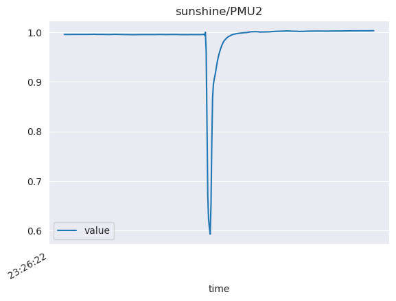
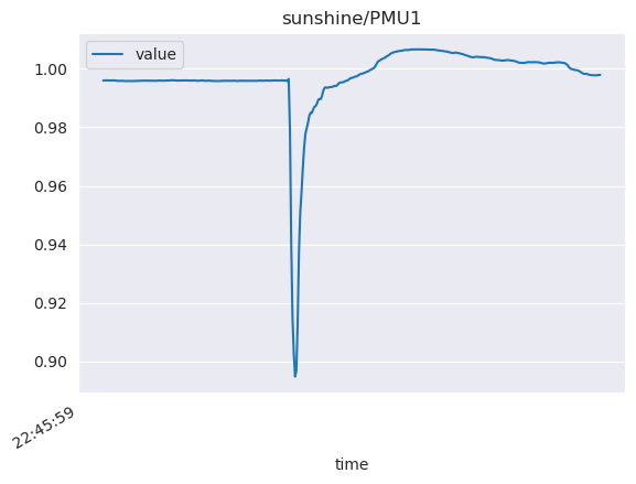
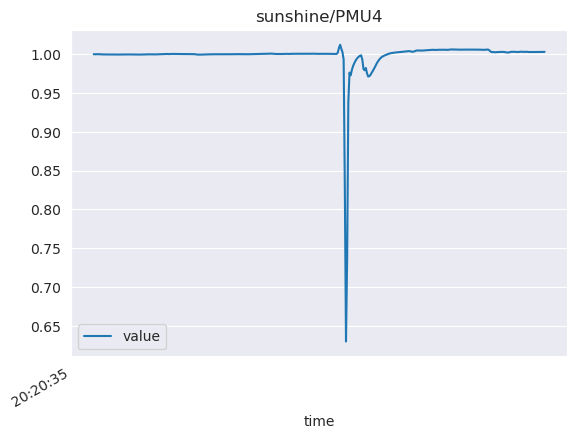
    print(f"For {key} A phase voltage mag, {len(stream_results)} sags found!")
    display(stream_results[-1].to_pandas().set_index("time").plot(title=f"{key}"))
For sunshine/PMU6 A phase voltage mag, 2 sags found!
<Axes: title={'center': 'sunshine/PMU6'}, xlabel='time'>
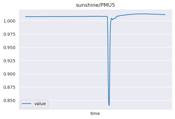
For sunshine/PMU5 A phase voltage mag, 50 sags found!
<Axes: title={'center': 'sunshine/PMU5'}, xlabel='time'>
For sunshine/PMU2 A phase voltage mag, 2 sags found!
<Axes: title={'center': 'sunshine/PMU2'}, xlabel='time'>
For sunshine/PMU1 A phase voltage mag, 16 sags found!
<Axes: title={'center': 'sunshine/PMU1'}, xlabel='time'>
For sunshine/PMU4 A phase voltage mag, 24 sags found!
<Axes: title={'center': 'sunshine/PMU4'}, xlabel='time'>
def merge_tables(data: dict[str, list[pa.Table]]) -> pd.DataFrame:
    # Convert each list of tables into a single concatenated table per key
    dfs = []
    for key, tables in data.items():
        concatenated_table = pa.concat_tables(tables)
        df = concatenated_table.to_pandas()
        df = df.rename(columns={"value": key})
        dfs.append(df)

    # Merge all dataframes on the 'time' column
    merged_df = dfs[0]
    for df in dfs[1:]:
        merged_df = pd.merge(merged_df, df, on="time", how="outer")

    return merged_df


def perform_correlation_analysis(merged_df: pd.DataFrame) -> pd.DataFrame:
    # Remove 'time' column for correlation analysis
    df = merged_df.set_index("time")
    correlation_matrix = df.corr()

    return correlation_matrix


# # Example usage
# data = {
#     "timeseries1": [
#         pa.table({"time": [1, 2, 3], "value": [10, 20, 30]}),
#         pa.table({"time": [4, 5], "value": [40, 50]}),
#     ],
#     "timeseries2": [pa.table({"time": [1, 3, 4], "value": [15, 25, 35]})],
#     "timeseries3": [pa.table({"time": [2, 3, 5], "value": [12, 22, 32]})],
# }

# merged_df = merge_tables(data)
# correlation_matrix = perform_correlation_analysis(merged_df)
# print(correlation_matrix)
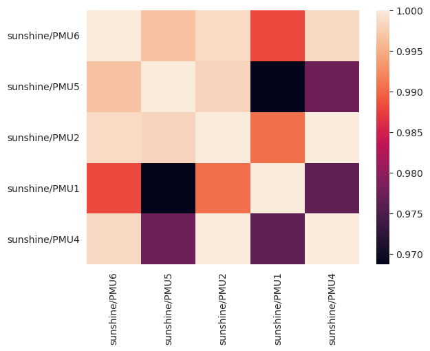
merged_df = merge_tables(result_dict)
corr_df = perform_correlation_analysis(merged_df)
corr_df
| sunshine/PMU6 | sunshine/PMU5 | sunshine/PMU2 | sunshine/PMU1 | sunshine/PMU4 | |
|---|---|---|---|---|---|
| sunshine/PMU6 | 1.000000 | 0.996615 | 0.998574 | 0.988252 | 0.998495 |
| sunshine/PMU5 | 0.996615 | 1.000000 | 0.998159 | 0.968694 | 0.977561 |
| sunshine/PMU2 | 0.998574 | 0.998159 | 1.000000 | 0.990526 | 0.999887 |
| sunshine/PMU1 | 0.988252 | 0.968694 | 0.990526 | 1.000000 | 0.976392 |
| sunshine/PMU4 | 0.998495 | 0.977561 | 0.999887 | 0.976392 | 1.000000 |
sns.heatmap(corr_df)
<Axes: >
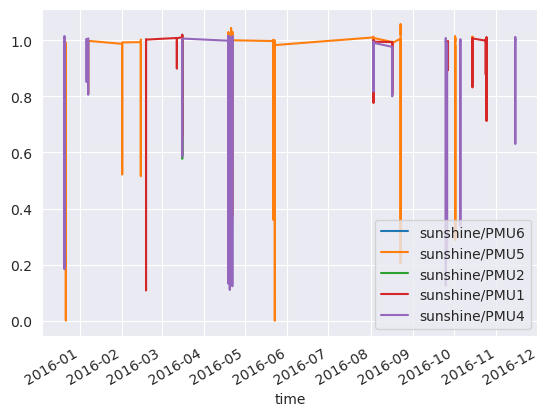
merged_df.set_index("time").plot()
<Axes: xlabel='time'>
Day of the week plot#
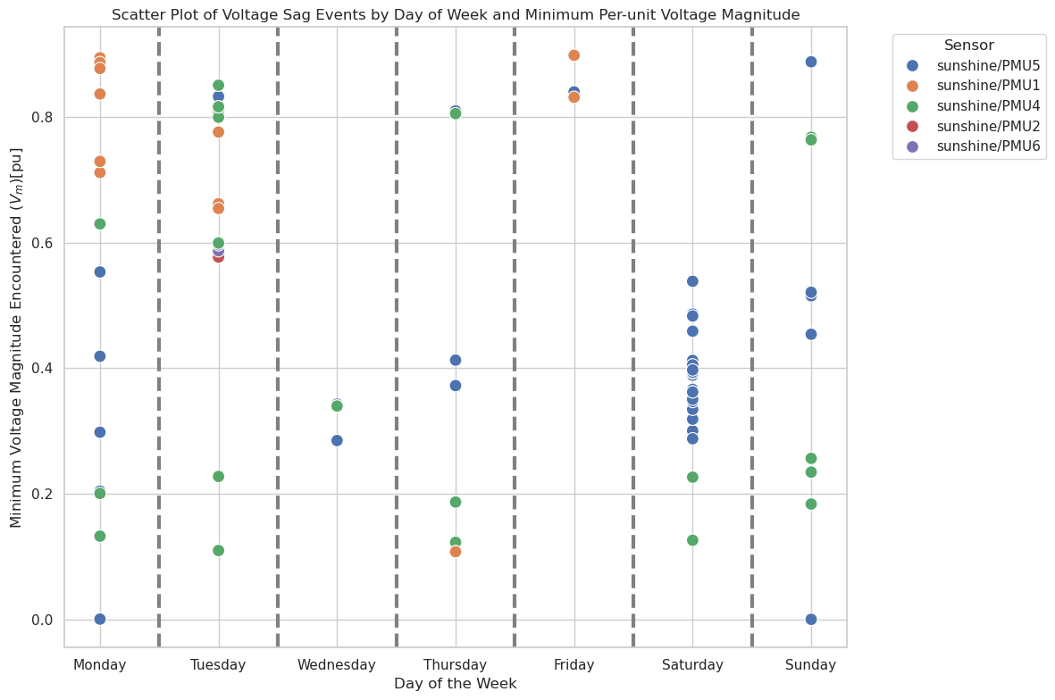
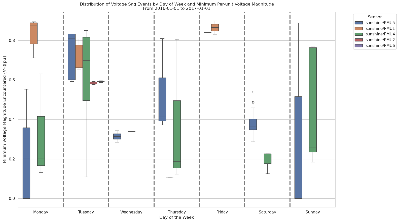
Since this is a distribution system being monitored, do these voltage sags occur most often on certain days of the week?
# iterate through each event (the list of tables), extract the day of the week 0->6 (monday->sunday) the event exists in
# take the average and assign it to the floor of that value, create a histogram
def extract_weekday_and_min_pu_value(tab: pa.Table) -> tuple[int, float]:
    weekday_vals = int(pc.mean(pc.day_of_week(tab["time"])).as_py())
    min_val_pu = pc.min(tab["value"]).as_py()
    return weekday_vals, min_val_pu
weekday_summary_dict = dict()
weekday_map = {
    idx: day
    for idx, day in zip(
        range(7),
        ["Monday", "Tuesday", "Wednesday", "Thursday", "Friday", "Saturday", "Sunday"],
    )
}
for collection, events in tqdm(result_dict.items()):
    days_values = list()
    for event in events:
        days_values.append(extract_weekday_and_min_pu_value(tab=event))
    weekday_summary_dict[collection] = days_values
weekday_data = [
    (coll, day, value)
    for coll in weekday_summary_dict.keys()
    for day, value in weekday_summary_dict[coll]
]
# weekday_data
weekday_df = pd.DataFrame(data=weekday_data, columns=["collection", "day", "value"])
weekday_df["weekday"] = weekday_df["day"].map(weekday_map)
weekday_df.astype(dtype={"collection": "category", "day": "string", "value": float})
weekday_df.sort_values(by="day", inplace=True)
# weekday_df.head()
# Create the plot
plt.figure(figsize=(16, 9))
sns.set(style="whitegrid")

# Create a scatter plot
scatter_plot = sns.boxplot(
    x="weekday",
    y="value",
    hue="collection",
    data=weekday_df,
)

# Add vertical lines to delineate weekdays
for i in range(1, 7):
    plt.axvline(x=i - 0.5, color="grey", linestyle="--", linewidth=3)

# Enhance the plot
plt.title(
    "Distribution of Voltage Sag Events by Day of Week and Minimum Per-unit Voltage Magnitude\nFrom 2016-01-01 to 2017-01-01"
)
plt.ylabel("Minimum Voltage Magnitude Encountered ($V_m$)[pu]")
plt.xlabel("Day of the Week")
plt.legend(title="Sensor", bbox_to_anchor=(1.05, 1), loc="upper left")

# Show the plot
plt.tight_layout()
plt.savefig("vsag_distribution_sunshine_data_2016_2017.png", dpi=200)
plt.show()
# Create the plot
plt.figure(figsize=(12, 8))
sns.set(style="whitegrid")

# Create a scatter plot
scatter_plot = sns.scatterplot(x="weekday", y="value", hue="collection", data=weekday_df, s=100)

# Add vertical lines to delineate weekdays
for i in range(1, 7):
    plt.axvline(x=i - 0.5, color="grey", linestyle="--", linewidth=3)

# Enhance the plot
plt.title(
    "Scatter Plot of Voltage Sag Events by Day of Week and Minimum Per-unit Voltage Magnitude"
)
plt.ylabel("Minimum Voltage Magnitude Encountered ($V_m$)[pu]")
plt.xlabel("Day of the Week")
plt.legend(title="Sensor", bbox_to_anchor=(1.05, 1), loc="upper left")

# Show the plot
plt.tight_layout()
plt.show()