Active and Reactive Power#

This notebook is intended as a quick start to working with data using PredictiveGrid’s Python API. It illustrates the inportant functionality of the API through performing a common power calculation.

The very first step is to import all the required packages. Below is a list of basic imports that you can copy and paste into your own notebooks to get going. The external python libraries (matplotlib, numpy, etc.) have wonderful, extensive documentation that you should look up if you want to explore all their functionalities or just unblock yourself. The %matplotlib inline command ensures that plots will be rendered in the notebook itself, rather than in a pop-up window.

# PredictiveGrid imports
import matplotlib.pyplot as plt  # plotting package

# External Python libraries
import numpy as np  # scientific computing package
import pandas as pd  # data analysis library
import pingthings as pt
import seaborn as sns  # pretty plotting package

sns.set_style("darkgrid")

Next, we must connect to the database. The connect function optionally accepts a profile string if you have multiple BTrDB configurations defined in your ${HOME}/.predictivegrid/credentials.yaml

>>> pt.connect(profile="my_cluster")

When running a notebook on JupyterHub, this does not need to be passed. Authenticating and logging into the predictive grid will happen based on variables encoded into the environment that pt.connect will look for when you pass nothing to connect()

conn = pt.connect()
print(f"{conn.info() = }")

conn.info() = {'major_version': 5, 'minor_version': 48, 'build': '5.48.0', 'proxy': {'proxy_endpoints': []}}

Power Calculation#

Lets compute active and reactive power from our phasor measurements from the sunshine dataset for 1 24Hr period.

We will calculate complex power at multiple points in time using the sunshine data. You can read more about the sunshine dataset on the blog here. You can find a diagram with approximate sensor locations here. This blog post introduces what complex power is, and of course you can find out more on wikipedia. Another relevant topic is the meaning of phasors which is introduced here.

We will do the following:

Grab current and voltage phasor streams (magnitude and angle)
Grab the status flag stream to use as a boolean mask
pick a 24 hr region of time and pull data
mask with the status flag
Compute phasors
compute a,b,c phase power
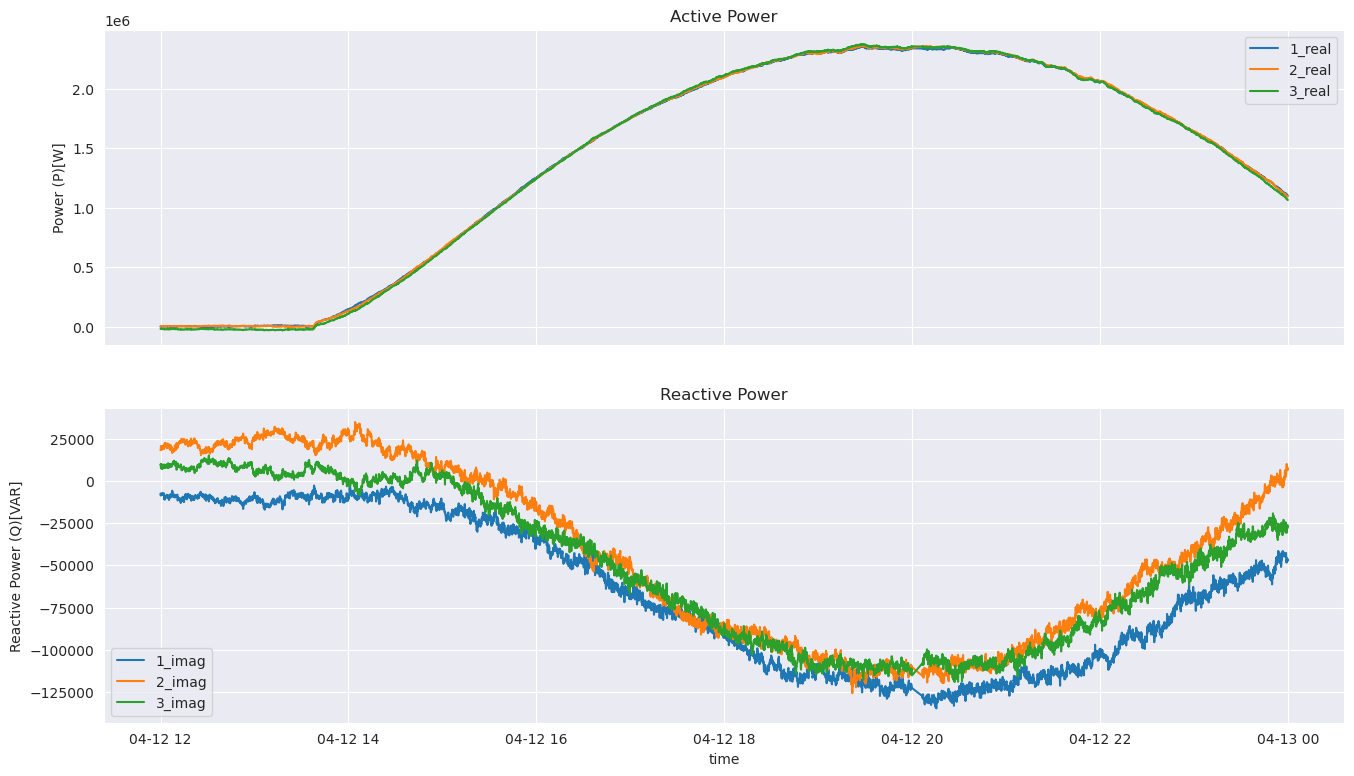
plot active and reactive power

1-2. Get phasor streams and statusflags#

sunshine_streams = conn.streams_in_collection("sunshine/PMU1", is_collection_prefix=False)
print(f"{sunshine_streams = }")
for stream in sunshine_streams:
    print(f"  - {stream.name}: {stream.uuid}")

sunshine_streams = <pingthings.timeseries.client.StreamSet object at 0x7e79a062f460>
  - C1MAG: 1187af71-2d54-49d4-9027-bae5d23c4bda
  - L2MAG: d4cfa9a6-e11a-4370-9eda-16e80773ce8c
  - C2MAG: d765f128-4c00-4226-bacf-0de8ebb090b5
  - L1ANG: 51840b07-297a-42e5-a73a-290c0a47bddb
  - LSTATE: 6ffb2e7e-273c-4963-9143-b416923980b0
  - L2ANG: 886203ca-d3e8-4fca-90cc-c88dfd0283d4
  - C1ANG: d625793b-721f-46e2-8b8c-18f882366eeb
  - C3ANG: 0be8a8f4-3b45-4fe3-b77c-1cbdadb92039
  - C3MAG: fb61e4d1-3e17-48ee-bdf3-43c54b03d7c8
  - L1MAG: 35bdb8dc-bf18-4523-85ca-8ebe384bd9b5
  - L3MAG: b2936212-253e-488a-87f6-a9927042031f
  - L3ANG: e4efd9f6-9932-49b6-9799-90815507aed0
  - C2ANG: 97de3802-d38d-403c-96af-d23b874b5e95

3. Pick a 12hr region of time and pull data#

start = pt.utils.to_nanoseconds("2017-04-12 12:00:00")
end = start + pt.utils.ns_delta(hours=12)

Here we’re using two helper functions, which can be conveniently found in our utils module.

sunshine_df = (
    sunshine_streams.raw_values(start=start, end=end)
    .to_pandas()
    .set_index("time")
    .rename(columns={str(s.uuid): s.name for s in sunshine_streams})
)
sunshine_df.info()

<class 'pandas.core.frame.DataFrame'>
DatetimeIndex: 5137440 entries, 2017-04-12 12:00:00.008333+00:00 to 2017-04-12 23:59:59.999999+00:00
Data columns (total 13 columns):
 #   Column  Dtype  
---  ------  -----  
 0   C1MAG   float32
 1   L2MAG   float32
 2   C2MAG   float32
 3   L1ANG   float32
 4   LSTATE  float32
 5   L2ANG   float32
 6   C1ANG   float32
 7   C3ANG   float32
 8   C3MAG   float32
 9   L1MAG   float32
 10  L3MAG   float32
 11  L3ANG   float32
 12  C2ANG   float32
dtypes: float32(13)
memory usage: 294.0 MB

4. Mask data with status flag#

sunshine_df.mask(sunshine_df["LSTATE"] != 0.0, inplace=True)
sunshine_df.dropna(inplace=True)
sunshine_df.drop(columns=["LSTATE"], inplace=True)
sunshine_df.head()

	C1MAG	L2MAG	C2MAG	L1ANG	L2ANG	C1ANG	C3ANG	C3MAG	L1MAG	L3MAG	L3ANG	C2ANG
time
2017-04-12 12:00:00.008333+00:00	1.067941	7193.234863	2.647526	210.967102	331.291412	287.297852	301.331329	2.655875	7199.367188	7161.541992	91.143814	258.771149
2017-04-12 12:00:00.016666+00:00	1.077288	7192.982422	2.649505	211.071106	331.393402	288.795532	301.874603	2.670920	7199.201172	7161.606445	91.246574	259.514709
2017-04-12 12:00:00.024999+00:00	1.074659	7192.908691	2.656754	211.170074	331.494598	288.327698	301.570648	2.663389	7198.952148	7161.555176	91.348557	259.207123
2017-04-12 12:00:00.033333+00:00	1.077025	7193.023438	2.649952	211.270355	331.597321	288.766693	301.581818	2.668463	7199.125977	7161.547852	91.451042	259.199921
2017-04-12 12:00:00.041666+00:00	1.098161	7193.195801	2.665421	211.374374	331.700378	288.478912	301.532227	2.688999	7199.190918	7161.669922	91.554207	259.336182

tmp_cols = sunshine_df.columns.str.extract("(^[A-Z])([1-3])(.*)", expand=True)
tmp_cols.columns = ["type", "phase", "mag_or_ang"]

multi_index = pd.MultiIndex.from_frame(tmp_cols)
multi_index

MultiIndex([('C', '1', 'MAG'),
            ('L', '2', 'MAG'),
            ('C', '2', 'MAG'),
            ('L', '1', 'ANG'),
            ('L', '2', 'ANG'),
            ('C', '1', 'ANG'),
            ('C', '3', 'ANG'),
            ('C', '3', 'MAG'),
            ('L', '1', 'MAG'),
            ('L', '3', 'MAG'),
            ('L', '3', 'ANG'),
            ('C', '2', 'ANG')],
           names=['type', 'phase', 'mag_or_ang'])

sunshine_df.columns = multi_index
sunshine_df

type	C	L	C	L		C			L			C
phase	1	2	2	1	2	1	3		1	3		2
mag_or_ang	MAG	MAG	MAG	ANG	ANG	ANG	ANG	MAG	MAG	MAG	ANG	ANG
time
2017-04-12 12:00:00.008333+00:00	1.067941	7193.234863	2.647526	210.967102	331.291412	287.297852	301.331329	2.655875	7199.367188	7161.541992	91.143814	258.771149
2017-04-12 12:00:00.016666+00:00	1.077288	7192.982422	2.649505	211.071106	331.393402	288.795532	301.874603	2.670920	7199.201172	7161.606445	91.246574	259.514709
2017-04-12 12:00:00.024999+00:00	1.074659	7192.908691	2.656754	211.170074	331.494598	288.327698	301.570648	2.663389	7198.952148	7161.555176	91.348557	259.207123
2017-04-12 12:00:00.033333+00:00	1.077025	7193.023438	2.649952	211.270355	331.597321	288.766693	301.581818	2.668463	7199.125977	7161.547852	91.451042	259.199921
2017-04-12 12:00:00.041666+00:00	1.098161	7193.195801	2.665421	211.374374	331.700378	288.478912	301.532227	2.688999	7199.190918	7161.669922	91.554207	259.336182
...	...	...	...	...	...	...	...	...	...	...	...	...
2017-04-12 23:59:59.966666+00:00	152.678528	7237.336914	150.528793	102.993713	223.317429	105.277977	344.750916	147.771149	7230.329590	7209.026367	343.269073	222.974060
2017-04-12 23:59:59.974999+00:00	152.694809	7237.402344	150.406143	102.986305	223.307922	105.280144	344.690491	147.859024	7230.400879	7209.247070	343.261108	222.920547
2017-04-12 23:59:59.983333+00:00	152.680252	7237.415039	150.426971	102.977066	223.299515	105.248222	344.674164	147.854050	7230.480469	7209.358398	343.253326	222.904129
2017-04-12 23:59:59.991666+00:00	152.613007	7237.575684	150.528397	102.966736	223.291412	105.233086	344.693695	147.851013	7230.523438	7209.407715	343.245300	222.870239
2017-04-12 23:59:59.999999+00:00	152.669434	7237.865723	150.483536	102.960045	223.285355	105.246346	344.675110	147.863663	7230.591797	7209.452637	343.240112	222.887329

5133840 rows × 12 columns

idx = pd.IndexSlice

5. Calculate Phasors#

def calc_phasors(mag: pd.Series, ang: pd.Series, unwrap: bool = True):
    if unwrap:
        ang = np.deg2rad(np.unwrap(ang.to_numpy().flatten()))
    else:
        ang = np.deg2rad(ang.to_numpy().flatten())
    return mag.to_numpy().flatten() * np.exp(1j * ang)

# angle goes from 0->360 here, not -pi <-> pi, not unwrapping
phasor_map = dict()
for type in ["C", "L"]:
    for phase in ["1", "2", "3"]:
        phasor_map[type + "_" + phase + "_" + "phasor"] = calc_phasors(
            mag=sunshine_df.loc[:, idx[type, phase, "MAG"]],
            ang=sunshine_df.loc[:, idx[type, phase, "ANG"]],
            unwrap=False,
        )

phasor_df = pd.DataFrame.from_dict(phasor_map)
phasor_df.index = sunshine_df.index

phasor_df

	C_1_phasor	C_2_phasor	C_3_phasor	L_1_phasor	L_2_phasor	L_3_phasor
time
2017-04-12 12:00:00.008333+00:00	0.317540- 1.019640j	-0.515548- 2.596844j	1.381019- 2.268581j	-6173.189941-3704.404053j	6309.000488-3455.305908j	-142.958572+7160.115234j
2017-04-12 12:00:00.016666+00:00	0.347094- 1.019841j	-0.482165- 2.605263j	1.410411- 2.268161j	-6166.313477-3715.518311j	6314.919434-3443.949463j	-155.801437+7159.911133j
2017-04-12 12:00:00.024999+00:00	0.337928- 1.020146j	-0.497501- 2.609757j	1.394416- 2.269195j	-6159.673340-3726.035645j	6320.927734-3432.755371j	-168.544006+7159.571777j
2017-04-12 12:00:00.033333+00:00	0.346495- 1.019767j	-0.496555- 2.603013j	1.397515- 2.273245j	-6153.290527-3736.900635j	6327.172852-3421.471680j	-181.350113+7159.251465j
2017-04-12 12:00:00.041666+00:00	0.348068- 1.041540j	-0.493225- 2.619388j	1.406287- 2.291958j	-6146.552246-3748.098389j	6333.468262-3410.167725j	-194.243622+7159.035156j
...	...	...	...	...	...	...
2017-04-12 23:59:59.966666+00:00	-40.231133+147.282684j	-110.136269-102.610527j	142.568344- 38.866180j	-1625.697266+7045.195312j	-5265.625977-4965.100586j	6903.848633-2075.315674j
2017-04-12 23:59:59.974999+00:00	-40.240990+147.296875j	-110.142227-102.424103j	142.612045- 39.039669j	-1624.802002+7045.475098j	-5266.497559-4964.271973j	6903.770996-2076.340332j
2017-04-12 23:59:59.983333+00:00	-40.155106+147.305222j	-110.186836-102.406715j	142.596115- 39.079018j	-1623.684448+7045.813965j	-5267.235840-4963.506836j	6903.595215-2077.310791j
2017-04-12 23:59:59.991666+00:00	-40.098518+147.250931j	-110.321724-102.410522j	142.606491- 39.029594j	-1622.423218+7046.148438j	-5268.054688-4962.872559j	6903.352539-2078.289551j
2017-04-12 23:59:59.999999+00:00	-40.147427+147.296097j	-110.258308-102.412895j	142.606033- 39.079178j	-1621.616089+7046.404785j	-5268.790039-4962.514648j	6903.206543-2078.927979j

5133840 rows × 6 columns

6. Compute Complex Power#

power_map = dict()
for phase in [1, 2, 3]:
    v_col = f"L_{phase}_phasor"
    c_col = f"C_{phase}_phasor"
    power_map[f"{phase}_power"] = phasor_df[v_col] * np.conj(phasor_df[c_col])

power_df = pd.DataFrame.from_dict(power_map)
power_df.index = phasor_df.index
power_df.head()

	1_power	2_power	3_power
time
2017-04-12 12:00:00.008333+00:00	1816.921387-7470.727051j	5720.296387+18164.871094j	-16440.730469+ 9563.940430j
2017-04-12 12:00:00.016666+00:00	1648.951172-7578.293945j	5927.558594+18112.580078j	-16459.572266+ 9745.038086j
2017-04-12 12:00:00.024999+00:00	1719.573242-7542.897461j	5813.987793+18203.886719j	-16481.486328+ 9600.960938j
2017-04-12 12:00:00.033333+00:00	1678.680542-7569.740234j	5764.343750+18168.666016j	-16528.173828+ 9592.909180j
2017-04-12 12:00:00.041666+00:00	1764.374634-7706.472168j	5808.727539+18271.792969j	-16681.369141+ 9622.460938j

7. Plot#

fig, ax = plt.subplots(nrows=2, ncols=1, figsize=((16, 9)), sharex=True)
ax[0].set_title("Active Power")
ax[1].set_title("Reactive Power")

ax[0].set_ylabel("Power (P)[W]")
ax[1].set_ylabel("Reactive Power (Q)[VAR]")

for phase in ["1", "2", "3"]:
    sns.lineplot(
        x=pd.DatetimeIndex(power_df.index[::1000]),
        y=np.real(power_df.filter(like=phase)[::1000].to_numpy().flatten()),
        ax=ax[0],
        label=f"{phase}_real",
    )
    sns.lineplot(
        x=pd.DatetimeIndex(power_df.index[::1000]),
        y=np.imag(power_df.filter(like=phase)[::1000].to_numpy().flatten()),
        ax=ax[1],
        label=f"{phase}_imag",
    )

../_images/b104788141e8078970e5ae60719fd27c9b2750404cb8aabc0a1a9a6a0c04094c.png

Active and Reactive Power

Contents